Using Machine Learning to Determine Conference Attendance From a Twitter Feed

Getting accurate information about conference attendance and participation is difficult. Available data feeds are not very accurate and do not provide the desired range of coverage at each included conference. Instead of relying on these feeds, ZoomInfo decided to use two alternate mechanisms for obtaining data to classify:

1. Scraping conference websites
2. Scraping Twitter feeds

This article discusses the second mechanism and how machine learning helps us better identify and interpret conference attendance data obtained via Twitter.

The Goal

ZoomInfo identified five possible types of conference attendees:

• attendee
• speaker
• sponsor
• exhibitor
• unknown

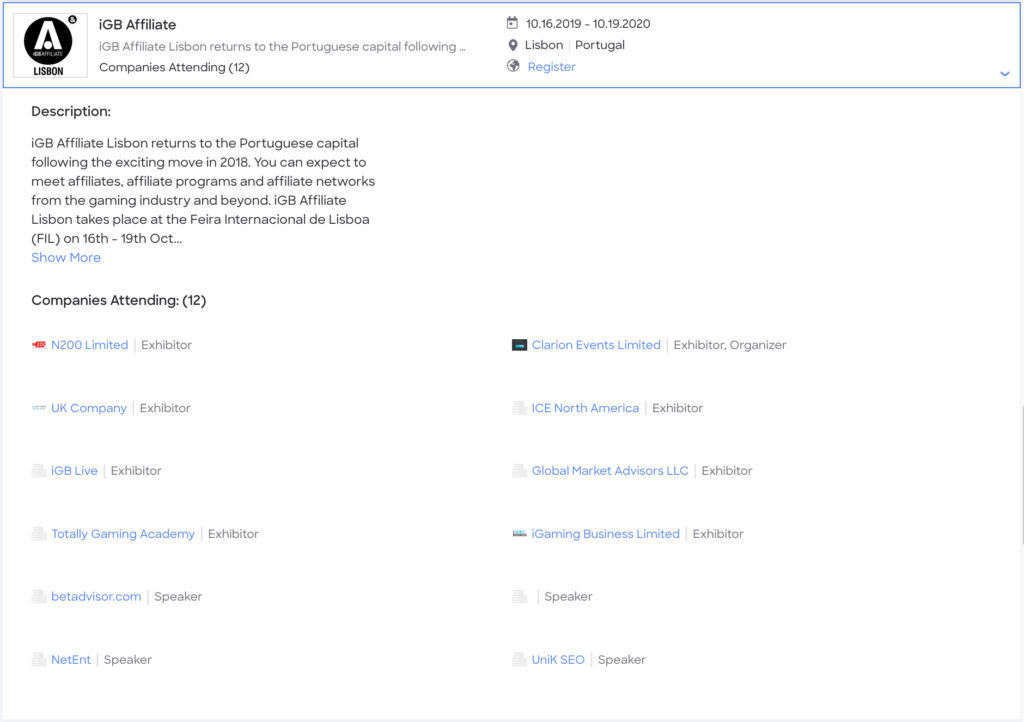
The goal of this project was to use the Twitter API to look for tweets that reference specific conferences using their official hashtags and classify any companies mentioned in the tweets into one of these categories. The company of the tweeter may also be identified, but usually only if they tweet from a work Twitter account or use a work email.

For example, in a tweet saying “I saw a demo by @foo”, ZoomInfo identified the @foo company as exhibitors and potentially identified the tweeter as an attendee. The tweeting account was then examined and if it belonged to a company that company was classified as an attendee. If the tweeter was identified as an individual but the account lists a recognizable corporate email account then the company owning that email domain was classified as an attendee at the conference. If the tweeter could not be identified or if the tweeter was an individual without a recognizable corporate email attached to their Twitter account, no attendee classification was made based on the tweet.

The General Approach

ZoomInfo applied a fairly standard machine learning approach to analyzing tweets:

1. Determine a ground truth data set
2. Preprocessing to standardize data
3. Modeling the Data
4. Implementing Algorithms to Classify New Data

Determining Ground Truth

Ground truth, or a set of data known to be accurately classified which can be used to learn how to classify other similar data, is a necessary starting point for machine learning. A ground truth set of data was identified by requesting tweets using a specific conference hashtag – #INBOUND18. A group of people manually identified the conference attendee type of each tweet’s author by comparing them to provided sample tweets for each possible category.

For example, the following tweet is an example of a speaker tweet:

Other tweets with the same context should also be classified as speaker tweets.

For better data accuracy, tweets were reviewed and labeled by multiple people. Initially two different people classified each tweet in the ground truth data set but that only resulted in agreement 80% of the time. This was not sufficient to reliably train the model to predict the attendee type. A second pass was made requiring at least four different people to examine and classify each tweet; most tweets were examined by exactly four people but some were looked at by five.

This second pass yielded better results by requiring greater agreement among the people evaluating the tweets. In this pass, only tweets where at least three of four or four of five people agreed on the classification were retained in the ground truth data; tweets that did not meet this threshold were removed. This ruled out tweets that had ambiguous context which might impede the model from learning. Approximately 13,000 tweets met the required threshold and were retained in the ground truth data set; of these just under 14% had three of four people agreeing on an assigned class, just under 1% had four of five people agreeing on an assigned class, and about 85% had all of the people examining them agree on an assigned class.

Standardizing the Data

One issue with classifying freeform tweets via automation is that there are many different ways to say the same thing. Identifying all of them as synonyms is nearly impossible. Instead, ZoomInfo grouped together similar words and phrases as things having the same meaning for purposes of analysis (for example, the following words all mean approximately the same thing and might get grouped together: sad, unhappy, melancholy, sorrowful, heartbroken, and disconsolate). It also identified similar relationships between sets of words such as groups of words that differ by the same single factor (for example, all of these word pairs differ solely by gender: man-woman, king-queen, brother-sister).

We also used a lemmatization process to identify different forms of the same root word and group them together as words with the same meaning. Lemmatization is a more advanced form of the common linguistics practice of stemming. Lemmatization not only identifies words that include the common stem or root word as part of the word itself (for example: walk, walked, walking, walks) but also identifies words with a common stem or root word that is not present in all forms of the word (for example: am, are, is are all forms of the common stem/root word be) and even distinguishes between homonyms (for example: left as in no longer present in a former location vs left as in a direction) when grouping words.

This preprocessing allows better correlation when doing automatic comparison of tweet contents to the identified ground truth set of tweet classifications during data modeling and determination of the efficacy of different algorithms.

Modeling the Data

After grouping like words together as outlined above, the next decision point was how to model the data to determine which words are meaningful when classifying tweets. The algorithms considered for this step include global vectors (GloVe) and term frequency-inverse document frequency (tf-idf). Once the meaningful words are chosen, the last step is to actually classify tweets by considering whether and how those words are included in various tweets. The algorithms considered for this step include long short term memory (LSTM), support vector machine (SVM) and gradient boosting.

The machine learning pipelines of algorithms considered for the two stages of this process fell in three lanes as follows:

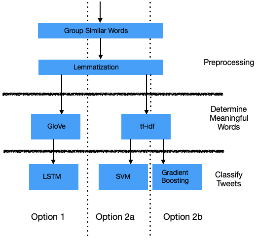
Option 1: Using GloVe and LSTM

The first option for modeling tweet classification includes using GloVe for determining the meaningful words and LSTM to take those words and determine how to classify the tweets into the five categories.

Using GloVe to Determine Meaningful Words

Global Vectors or GloVe uses a log-bilinear model to determine meaningful words by examining how often groups of words appear near each other in a large collection of related text. The key mechanism of GloVe is a word co-occurrence matrix, a matrix that records how often each word in the collection of text appears near each other word. This matrix is used to look at the relative likelihood of particular words to appear in conjunction with one word versus another – basically, the ratios of the probabilities of concurrence – and translates them into a word vector space to determine whether their pairing is meaningful or random.

Applying this technique to the text of available tweets identifies sets of words that have meaning and can be used to further evaluate the likely classification of each tweet in further steps of the process.

Using LSTM with Word Embedding

Long Short Term Memory or LSTM is a form of a recurrent neural network designed to retain important information for long periods of processing. It essentially chains together short-term decisions so that the important consequences of previous decisions trees are retained and considered in each new decision. This allows data processed many iterations ago to remain relevant while considering new data in fairly atomic, easy to process ways. Input gates are used to present the remembered data to a new decision gate containing the next piece of information, then the logic in that gate determines which information to retain moving forward and which information to forget. The output of this decision gate becomes the input gate of the next decision gate until all of the data is processed.

More information on LSTM is available in this article by Chris Olah.

ZoomInfo used this process with embedded words, bringing forward important words in tweets for comparison with later language to determine context and combinations of words that are more likely to indicate tweets belonging to a specific classification group.

Option 2a: Using tf-idf and SVM

The second option for modeling tweet classification includes using tf-idf for determining the meaningful words and SVM to take those words and determine how to classify the tweets into the five categories.

Using tf-idf to Determine Meaningful Words

Another option for tweet classification is using term frequency–inverse document frequency or tf-idf. Most commonly used in search engine scoring, this algorithm determines a relevancy score for each word in an entire data set based on its frequency in a particular document compared to the overall number of documents the word appears in. This is effectively a weighted comparison of word usage normalized against the general popularity of each word. Basically, the inclusion of a word in a document is judged against how likely that word is to appear in the average document in the data set.

In this case, each tweet is a document while the set of tweets within the ground truth data tagged with each classification option is treated as a separate full data set. When ZoomInfo ran a tf-idf analysis on the ground truth data, we discovered that many of the tweets included very strong correlations between specific words and the tweet classification. For example, the word “booth” appears very frequently in exhibitor tweets.

Words with a high frequency in one specific class of tweet may also appear in a much smaller (but still somewhat meaningful) percentage of tweets belonging to another class and appear very rarely if at all in other classes of tweets. The specific frequencies of each word’s usage in each class of tweets become relevancy scores that can later be assigned when a scored word appears in a tweet; the relevancy score for each word appearing in a specific tweet is combined to inform its classification.

Using Support Vector Machine to Classify Tweets

Support Vector Machines (SVMs) are algorithms that look to classify data points into one of two groups, finding the largest margin between the two groups. Since this is fundamentally a comparison of two options, the five tweet classes were grouped into their ten unique pairs (basic combinatorics tells us that there are 5!/(2!(5-2)!)=120/(26)= 120/12=10 unique pairs of five items). Let’s assign each of the five classes to a letter from A-E. These ten pairs are then:

{A,B},{A,C},{A,D},{A.E}

      {B,C},{B,D},{B,E}

            {C,D},{C,E}

                  {D,E}

To pick a single class by evaluating pairs, start with the binary choice of A or B (the first set of pairs) and pick a winner using SVM. The loser of the pairing is ruled out and all other pairs containing that option are removed from consideration. Move to the next remaining pairing (either {A,C} or {B,C}) and pick a winner of that pair using SVM. Again, remove all other pairs containing the loser from consideration and move to the next cell ({A,D} or {B,D} or {C,D}) and pick a winner of that pair. Remove all other pairs containing the loser from consideration and move to the last remaining cell ({A,E} or {B,E} or {C,E} or {D.E}). Pick the winner of this last pair and it becomes the classification for that tweet.

For example, let’s say a particular tweet is classified as A when using SVM on the {A,B} pairing. The {B,C}, {B,D}, and {B,E} pairs are ruled out, leaving the following pairs still to be evaluated:

{A,C},{A,D},{A.E}     

      {C,D},{C,E}

            {D,E}

When evaluated against the {A,C} pair, that same tweet is classified as C. The {A,D} and {A,E} pairs are ruled out, leaving the following pairs still to be evaluated:

{C,D},{C,E}

      {D,E}

When evaluated against the {C,D} pair, that same tweet is classified as C. The {D,E} pair is ruled out, leaving just the {C,E} pair to be considered. When the {C,E} pair is evaluated, the tweet is again classified as C which becomes the actual classification of the tweet.

Option 2b: Using tf-idf and Gradient Boosting

The third option for modeling tweet classification includes using tf-idf for determining the meaningful words and XGBoost to take those words and determine how to classify the tweets into the five categories.

Using tf-idf to Determine the Meaningful Words

The process for using tf-idf to determine meaningful words remains the same regardless of which algorithm follows for tweet classification; the discussion under Option 2a remains applicable in this option too and will not be repeated.

Using Gradient Boosting to Classify Tweets

Gradient Boosting, or more specifically Python’s XGBoost variant, takes weak correlations (correlations that are only slightly better than random grouping) and boosts them so they become stronger correlations that better predict results. It is an ensemble learning model, meaning that it combines small tests of data sequentially in ways that build on the information learned in previous tests.

Gradient boosting does this by emphasizing and putting additional weight on previous analysis that shows high errors or wrong predictions while also defining and trying to minimize a loss function (the first part of this is the boosting while the second is the gradient). This seems counterintuitive, but the idea behind putting additional weight on the errors is that the difficult cases and outliers will get the focus during the learning process and thus be handled better than if all input data was treated equally. Basically a prediction is made and compared to the expected results from ground truth data. A gradient is calculated based on a loss function representing the rate of error in the comparison to ground truth. This gradient guides the next round of predictions as attempts are made to minimize their number and size and the process is repeated. Each subsequent round of predictions is faster as the gradient is refined until all data is adequately classified.

More information on Gradient Boosting is available here or here.

Comparing the Three Options

Once the three possible options were identified and investigated, the results were analyzed to determine the best possible pipeline of algorithms to use to classify conference tweets into the five categories. This choice was made in two stages: 1) Determine if there’s a clear best option for determining the meaningful words in a tweet and 2) Determine the best option for classifying tweets using those meaningful words. If the two options for determining the meaningful words were approximately equal or if GloVe was a clear winner, all three possible tweet classification algorithms would be considered in the stage two comparison. However, if tf-idf is clearly a better option than GloVe then only SVM and gradient boosting will be compared (the two options that follow after using tf-idf for the first stage of determining the meaningful words).

Choosing Between Option 1 and the Two Option 2s: Comparing GloVe and tf-idf

The tf-idf approach to determining the correlation between specific words and likely tweet classification turned out to be up to five times more effective than the GloVe approach for the ZoomInfo data set. The largest difference in effectiveness is seen in those classes with the lowest quantity of ground truth data, so ZoomInfo speculates that this GloVe would approach or improve on the effectiveness of tf-idf with a sufficiently large ground truth data set.

However, with the ground truth set we used, tf-idf was definitely superior and thus the method we used to determine which words to consider in tweet classification.

Choosing Between Options 2a and 2b: Comparing SVM and XGBoost

Although the results were close, XGBoost resulted in slightly better results when comparing the F1 score for each algorithm (0.86 vs 0.84). This score is effectively a comparison of how well the results correlate to the known ground truth data classifications. Thus, ZoomInfo used Option 2b with tf-idf and XGBoost in its production model.

Implementing the Algorithms

The algorithms were implemented as two separate components: a trainer and a predictor.

Implementing the Trainer Component

The trainer was designed to retrain the model with new data to detect new patterns or when new ground truth data is obtained. Basically, this trainer constantly reconsiders the word grouping mechanisms in the preprocessing step and the identification of meaningful words used to seed the algorithms actually classifying tweets. ZoomInfo implemented this with Google’s ML engine to take advantage of its easy management features and scalability.

Implementing the Predictor Component

The Predictor component is a pipeline for receiving and classifying new tweets from the Twitter API. It is implemented as a REST API endpoint using Google’s App Engine to take advantage of quick deployment features and scalability.

Final Thoughts

While not perfect, ZoomInfo was able to use machine learning to develop a mechanism for identifying and classifying company attendance at technical conferences using Twitter hashtags associated with the conferences. The DiscoverOrg and ZoomInfo combined platform web application uses the results to display conferences and their identified attendees on its Events page.

This process has been in place for about nine months and has enhanced our ability to report on company conference attendance.